Land cover classification by remote sensing

The main objective of this project was to explore the automation of land cover classification based on multiple spectral bands from satellite imagery through the construction of a function. The function created is capable of performing unsupervised and supervised classifications. Allowing validation by comparison with observations, if possible, was the secondary objective of this function. This objective is completed by the calculation of some usual performance indices which are a confusion matrix and the associated kappa index. It should be noted that this personal project focused more on exploring automation in the context of remote sensing than on classification results per se. Although it already shows great results, the first case study could easily have been improved with a larger training database. The second case study deepens the automation process by leveraging an open land cover database. The results obviously depend heavily on the quality, quantity and diversity of the observations. The objective here is to demonstrate that a certain level of automation has been achieved and that the results could be easily improved only by having access to one or more additional databases and by choosing more carefully satellite images.

Workflow

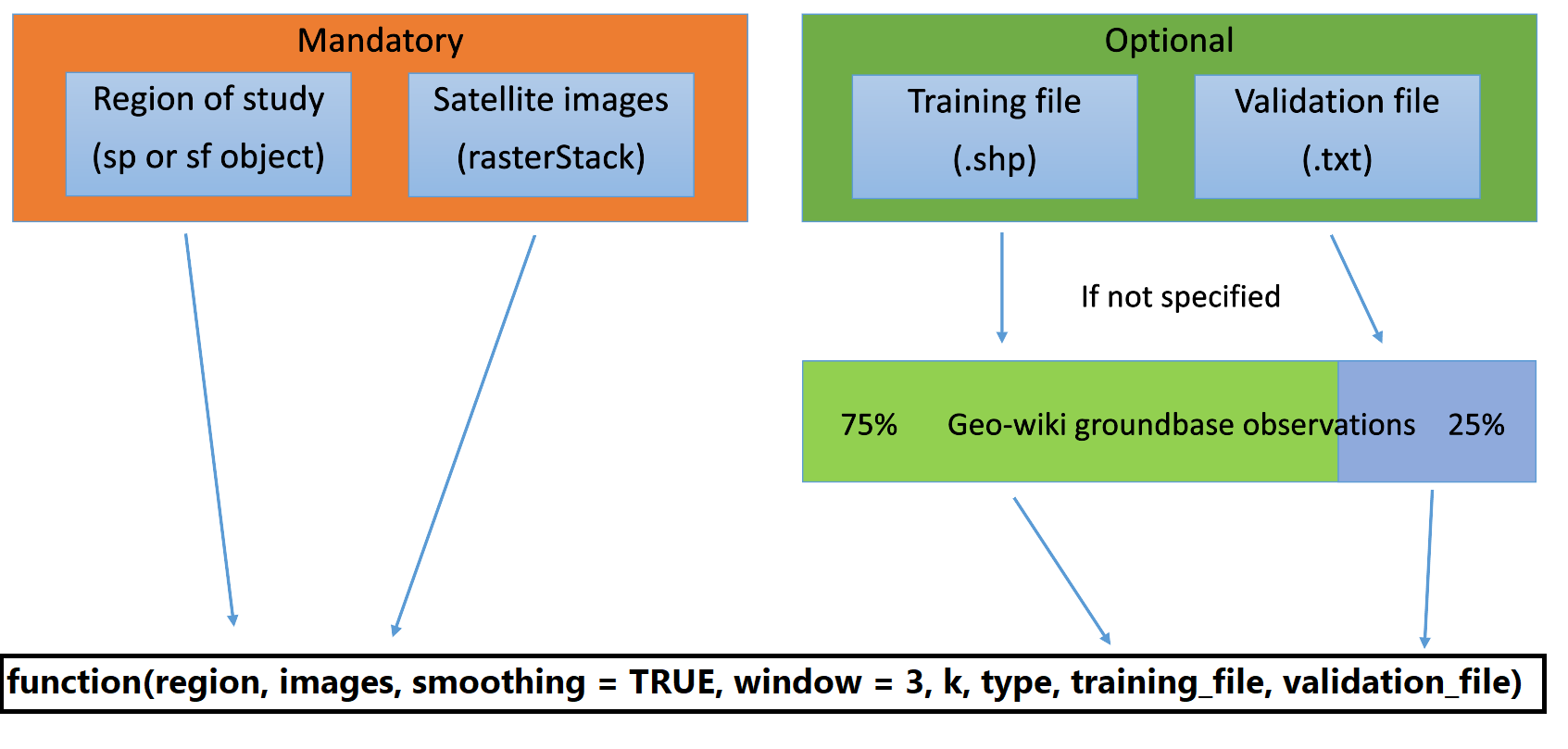
classification() function requires at least two mandatory inputs to run: a rasterStack composed of different relevant spectral bands and a spatial object (from sp or sf packages) delimiting the study region. The function can be completed with optional inputs which are a shapefile with training area, i.e. polygons assigned to the class actually observed (necessary for the supervised classification) and a validation text file. In case these two elements are not specified, the function searches in the geo-wiki ground based observations database (https://doi.pangaea.de/10.1594/PANGAEA.869682, Fritz et al, 2016 ) to check if there is enough data for the study region to replace the missing arguments.

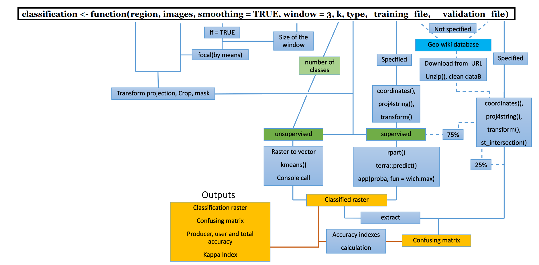
Concerning the processing, the first step is the smoothing of the satellite images via the focal() function. This first step benefits from the paralellization. Then the spatial object delimiting the region is reprojected to match the projection of the images. These are cropped and masked by the region object.

The classification is then carried out. In the case of the unsupervised algorithm (via the kmeans() function) tries to gather similar cells, ie close to each other in the multiple space where each dimension is a spectral band. For this, the raster must be transformed into a vector where each element corresponds to a cell of the raster. Finally, a console call to the user is made to assign the different groups to their land cover class. Note that, for an unsupervised classification, it is generally recommended to request more land cover classes than necessary and to regroup some of them after classification (methodological advice, not related to this specific project and function). The desired number of classes is chosen with the k argument.

Regarding supervised classification, if the training file is given, it is transformed into a spatial object by coordinates(). The object is then reprojected so that its projection matches that of the images. In case the file is missing, the geo wiki database is downloaded from the URL, unzipped and all unnecessary information is removed so that the file is finally a clean table. Then, it undergoes the same steps as a training file that would have been specified but also an intersection() function so that only the observations of the region studied remain. Only 75% of the observations will be used to perform the classification, the remaining 25% will be used for validation. The supervised algorithm (via the rpart() function) attempts to find a specific spectral signature for each class. The classes are separated by a "classification tree" from which is calculated the probability that each cell belongs to each class (via the predict() function). Finally, the cell is assigned to the class to which it has the highest probability of belonging.

In case a validation file is provided or there is enough data in the geo wiki database for the given region, the classification values ​​are extracted from the observation point locations and observations and predictions are combined in the same dataframe. From this data frame is created a confusion matrix which is a table comparing the predicted classes with the actual classes. Observations in the diagonal of the matrix are well classified. From this matrix, the producer, the user, the total accuracy and the kappa index are calculated. This last index measures the accuracy of the classification considering the possibility of agreement resulting from luck. See the comments in the code for detailed step-by-step explanations.

The final outputs are therefore the classified raster, the confusion matrix and the kappa index.

Code

library(raster)
library(rgdal)
library(sp)
library(sf)
library(dplyr)
library(RColorBrewer)
library(terra)
library(rpart)
library(parallel)
library(foreach)
	
classification <- function(images,  region, type, country, k, training_file, smoothing = TRUE, window = 3 , validation_file){
	#DESCRIPTION: create a land cover classification based on satellite images and compute validation indices
	#INPUTS: #images (RasterStack) with all satellite images which will be used
	  #type (character): 2 available types of classification: 'unsupervised' or 'supervised'
	  #region is a (SpatialPolygonsDataFrame sp or sf) used to mask images
		#region is dominant on country if both are specified
	  #country (character) specifying the ISO code of a country used to mask images
		#for countries smaller than the extent of images
	  #k (integer) is the number of classes for the unsupervised classification
	  #training_file (character) is the name of a shp file, in the current folder, used to perform the supervised classification
		#if training_file is not specified, then the geo-wiki ground observations database is used
		#see https://doi.pangaea.de/10.1594/PANGAEA.869682 (Fritz and al, 2016)
	  #smoothing (logical), default= TRUE
	  #window (integer) is the size of the smoothing window (odd number), i.e the intensity of the smoothing
	  #validation_file (character) is the name of a text file, in the current folder, with header of, at least, 4 columns called ID,lat,long,class
		#if validation_file is not specified, then the geo-wiki ground observations database is used
	#OUTPUTS: classified raster, confusion matrix, kappa index  and a character linking values of the classification with associated names of class
	
	#smoothing
	if (smoothing==TRUE){
	  #this step is the only one that can benefit from the parallelization
	  doParallel::registerDoParallel(parallel::detectCores()/2)
	  smooth<-foreach (i=1:nlayers(images)) %dopar%{
		#smoothing of each band with the window chosen
		terra::focal(images[[i]], w= matrix(1,window,window), mean)
	  }
	  images<-stack(smooth)
	  #stop parallelization to release RAM
	  doParallel::stopImplicitCluster()
	}
	#region of study
	if(missing(region)) {
	  if(missing(country)) {
		print('You did not specified a country or a region to mask')
	  } else {
		region <- raster::getData("GADM", country = country, level =0, download=TRUE)
	  }
	}
	#need sf class to perform some of the following steps
	region_sf<-st_as_sf(region)
	#match the projection of the region to that of the images
	region_sf<-st_transform(region_sf, crs(images))
	#cropping before most of the processing
	images_crop<-crop(images, region_sf)
	#note that the smoothing still need to be done before
	
	#import observations that will be used to validate (and used as training points in the case of supervised classification,
	#explaining why it is done before the classification)
	if(missing(validation_file)) {#if no validation file, the function will use the geo wiki ground observation database
	  print('Using geo wiki ground observation database, in case there is enough data for the region')
	  if (file.exists("datasets")==FALSE){ #avoid unnecessary download if it has already be done previously
		#download the zip file from the url
		download.file('https://doi.pangaea.de/10.1594/PANGAEA.869682?format=zip', "Fritz_2016.zip",mode="wb")#mode 'wb' for zip file
		unzip( "Fritz_2016.zip")
	  }
	  #the raw file is not directly useable, need to skip 'metadata information' lines
	  obs<-read.table('datasets/GlobalCrowd.tab', header = F, na.strings= "",sep = "\t", dec = ".", fill=T, skip=34)
	  #if v20 is na, this means that the observation is for the day it was implemented
	  #otherwise v20 is specified
	  #combine to keep only the information related to the date that has been used to classify, not the date when the classify has be perform
	  obs[!is.na(obs$V20),]$V19<-obs[!is.na(obs$V20),]$V20
	  #keep only the obs with a strong confidence v8 on the class(given by the geowiki user) (at least 90% confidence)
	  obs<-obs[obs$V8>=90,]
	  #keep useful columns only
	  obs<-dplyr::select(obs,V4,V5,V7,V19)
	  #keep the year of observation
	  obs$V19<-substr(obs$V19,1,4)
	  #rename columns
	  colnames(obs)<-c('long','lat','nb_class','date')
	  #an ID without missing number will be useful for some of the following steps
	  obs$ID<-1:nrow(obs)
	  #correspondence between number and class (information from the metadata)
	  geo_wiki_occup<-c('treecover','shrubcover','grassland','cultivated','mosaic','wetland','urban','snoworice','barren','water')
	  obs$class<-geo_wiki_occup[obs$nb_class]
	  
	} else {
	  #using the validation file specified by the user
	  obs<-read.table(validation_file, header = TRUE, sep = ",", dec = ".")
	}
	
	#transform observation file in a spatial object
	sp::coordinates(obs)<-~long+lat
	#set the right projection (gps)
	proj4string(obs)<-crs("+proj=longlat +datum=WGS84 +no_defs")
	#need sf class to perform some of the following steps
	obs_sf<-st_as_sf(obs)
	#match the projection of the observations to that of the images
	obs_sf<-st_transform(obs_sf, crs(images))
	#keep only observations points in the region
	obs_sf <- st_intersection(obs_sf, region_sf)
	#need sp class to perform some of the following steps
	obs<-as(obs_sf, 'Spatial')
	
	#CLASSIFICATION#
	
	if(type=='unsupervised'){ #UNSUPERVISED
	  #transform the rasterStack information into a numeric object (required for the kmeans()function)
	  values<-getValues(images_crop)
	  #algorithm which gather similar cells and segregate cells that are different
	  kmn <- kmeans(na.omit(values), centers = k, iter.max = 500, nstart = 5, algorithm="Lloyd")
	  #set the information as a raster
	  knr <- setValues(images_crop, kmn$cluster)
	  #only the first element is useful
	  knr <- knr[[1]]
	  # mask
	  classification<-mask(knr,region_sf)
	  #the classification is plotted to allow the user to assign classes
	  mycolor <- brewer.pal(k, "Set3")
	  plot(classification, main = 'Unsupervised classification', col = mycolor )
	  
	  #ask the user to assign classes
	  occup<-NULL
	  print('on the basis of the map, associate the number to its class')
	  print('different numbers can be associated to the same name of class')
	  if(missing(validation_file)){
		#inform on the class names used in the geo wiki database
		print('available classes are: treecover, shrubcover, grassland, cultivated, mosaic, wetland, urban, snoworice, barren, water')
	  } else {
		print('respect the class names given in your validation file')
	  }
	  for (i in 1:k){ #console call to the user
		occup[i] <- readline(prompt=paste0("Class ",i," is: "))
	  }
	  
	} else if(type=='supervised'){ #SUPERVISED
	  if(missing(training_file)){ #unsupervised by using geo wiki ground observation database
		# we will use the already downloaded geo wiki ground observations as training points
		#only 75% of data, 25% rest will be used for the validation
		ptsamp<-obs[1:(round(0.75*nrow(obs))),]
	  } else { #unsupervised by specified training file
		#download training points file
		shape <- readOGR(dsn = ".", layer = training_file)
		#match the projection to that of the images
		shape<-spTransform(shape, crs(images_crop))
		#the supervised algorithm need points to work, so we generate point samples inside the polygons
		ptsamp <- spsample(shape, 1000, type='random')
		# save the information on the class
		ptsamp$class <- over(ptsamp, shape)$class
	  }
	  if(nrow(ptsamp)>10){#a minimum of training points is required to perfom the classification
		df <- extract(images_crop, ptsamp )
	  }else{
		print('not enough observations to perfom a classification for this region')
	  }
	  #data frame containing information for each point for each band and class
	  sampdata <- data.frame(class = ptsamp$class, df)
	  #some of the following steps require the raster to be a "SpatRaster" object from 'terra' package
	  images_crop<-as(images_crop, "SpatRaster")
	  #the model requires the classes to be factor to work properly, not character
	  #we save the information linking classes to factor into a dataframe used later
	  a<-data.frame(class = unique(sampdata$class), code=1:length(unique(sampdata$class)))
	  #give the same name as the object resulting from the unsupervised==T if statement
	  occup<-a$class
	  #assign the corresponding number for each observation
	  sampdata$class_code<-NULL
	  for (i in 1:nrow(sampdata)){
		sampdata$class_code[i]<-a[a$class==sampdata$class[i],]$code
	  }
	  # Train the model 
	  model <- rpart(class_code~., data = sampdata[2:length(sampdata)], method = 'class')#, minsplit = 5)
	  #classification tree
	  plot(model, uniform=TRUE, main="Classification Tree")
	  text(model, cex = 1)
	  #predict, by using the model, the probability of cells to belong to each class
	  proba <- terra::predict(images_crop, model, na.rm = TRUE)
	  #multiple maps giving the probability of each cell to belong to each class
	  plot(proba)
	  #assign to each cell the class for which it has the max probability of belonging
	  classification <- app(proba, fun = which.max)
	  #mask
	  classification<-raster(terra::mask(classification,as(region_sf, "SpatVector")))
	  #plot the resulting map
	  mycolor <- brewer.pal(length(unique(sampdata$class)), "Set3")
	  plot(classification, main = 'supervised classification', col = mycolor)
	}
	
	#VALIDATION
	#extraction of the value predicted by the classification for each validation point
	#class of object depends on the classification type and therefore requires a different extracting function
	if(type=='unsupervised'){
	  df <- extract(classification, obs_sf, df=TRUE)
	} else if(type=='supervised'){
	  if(missing(training_file)){#in this situation, the 25% of observations not used to perform the model will evaluate it
		obs<-obs[(round(0.75*nrow(obs))):nrow(obs),]
		df <- extract(classification, obs, df=TRUE)
	  } else {
		df <- extract(classification, obs_sf, df=TRUE)
	  }
	}
	#combine result of the classification with observation data
	obs$nb_classif<-df[,ncol(df)]
	#associate class name to the number on the basis of occup object
	#for the unsupervised classification: occup is defined by the console call to the user
	#for the supervised classification: occup comes from the 'backup dataframe = a'
	obs$class_classif<-occup[obs$nb_classif]
	
	
	if (nrow(obs)>=10){ #number of observations threshold to perform a validation
	  #confusion matrix where row names are actual classes and column names are classes predicted by the classification
	  confusion<-matrix(0,length(unique(occup)),length(unique(occup)), dimnames = list(unique(occup),unique(occup)))
	  for (i in 1:nrow(obs)){
		confusion[rownames(confusion)==obs$class[i],colnames(confusion)==obs$class_classif[i]]<-(confusion[rownames(confusion)==obs$class[i],colnames(confusion)==obs$class_classif[i]])+1
	  }
	  #total accuracy index
	  total_accuracy<-sum(diag(confusion))/sum(confusion)
	  #kappa index
	  off_diag<-1-total_accuracy
	  kappa_index<-(total_accuracy-off_diag)/(1-off_diag)
	  #inclusion index
	  inclusion_error<-NULL
	  for (i in 1:ncol(confusion)){
		inclusion_error[i]<-confusion[i,i]/sum(confusion[,i])
	  }
	  #exclusion index
	  exclusion_error<-NULL
	  for (i in 1:nrow(confusion)){
		exclusion_error[i]<-confusion[i,i]/sum(confusion[i,])
	  }
	  #bind total accuracy, inclusion and exclusion indexes to the confusion matrix
	  confusion<-rbind(confusion,inclusion_error)
	  confusion<-cbind(confusion,exclusion_error)
	  confusion[nrow(confusion),ncol(confusion)]<-total_accuracy
	} else {
	  print('not enough observations to perform a validation')
	  #return at least the classification
	  return(classification)
	}
	#return the ouptuts
	outputList <- list("classification" = classification, "kappa_index" = kappa_index, "confusion_matrix" = confusion, 'class_order'= occup)
	return(outputList)
  }

First case study: Brabant Wallon (with optional inputs)

In the first example, we will carry out a land cover classification in the Brabant Wallon region using optional inputs. First, all bands from a set of Landsat 5 images are imported and stacked. A spatial object for the region is also downloaded.

#import and stack satellite images
landsat<-stack()
for (i in 1:7){
	name <- paste0('landsat',i)
	assign(name, raster(paste0('images/LT05_L1TP_198025_20090530_20200827_02_T1_B',i,'.tif')))
	landsat<-stack(landsat,eval(parse(text=name)))
}

#import spatial object for the region of study
belgium <- raster::getData("GADM", country = 'BEL', level =2, download=TRUE)
belgium_sf<-st_as_sf(belgium)
bw_sf<-belgium_sf[7,7]

Then we call the function specifying the unsupervised classification and providing the optional input which is the validation file.

#call function with optional arguments for unsupervised classification
output<-classification(images=landsat,region = bw_sf, smoothing = TRUE, window = 3, type = 'unsupervised', k=4,validation_file = 'points.txt')
output
#plot
plot(output[[1]], main='Unsupervised classification of Brabant Wallon', legend = FALSE, col = c("#70C108",'#E4811D','#FBF463','#AEE41D'))
legend("topright", legend = output[[4]], fill = c("#70C108",'#E4811D','#FBF463','#AEE41D'))

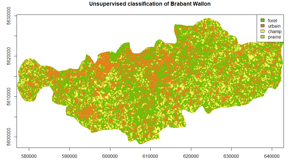
For someone who knows the region a little, it is clear that the classification underrepresents the fields in favor of the forests. These results could have been easily improved, for example by choosing more than 4 classes and then grouping them together. Again, that was not the point here.

Now we call the function specifying the supervised classification and providing the optional inputs

#call function with optional arguments for supervised classification
output<-classification(images=landsat, region = bw_sf, smoothing = TRUE, window = 3, type = 'supervised', training_file = "training",validation_file = 'points.txt')
output

## $classification
## class      : RasterLayer 
## dimensions : 1040, 2199, 2286960  (nrow, ncol, ncell)
## resolution : 30, 30  (x, y)
## extent     : 576945, 642915, 5598195, 5629395  (xmin, xmax, ymin, ymax)
## crs        : +proj=utm +zone=31 +datum=WGS84 +units=m +no_defs 
## source     : memory
## names      : lyr.1 
## values     : 1, 4  (min, max)
## 
## 
## $kappa_index
## [1] 0.8181818
## 
## $confusion_matrix
##                 champ urbain prairie foret exclusion_error
## champ             3.0      0       0     0       1.0000000
## urbain            0.0      4       0     0       1.0000000
## prairie           1.0      0       2     0       0.6666667
## foret             1.0      0       0     2       0.6666667
## inclusion_error   0.6      1       1     1       0.8461538
## 
## $class_order
## [1] "champ"   "urbain"  "prairie" "foret"

#plot
plot(output[[1]], main='Supervised classification of Brabant Wallon', legend = FALSE, col = c('#AEE41D','#FBF463',"#70C108",'#E4811D'),xlab = "Longitude (m)",  ylab = "Latitude (m)")
legend("topright", legend = output[[4]], fill = c('#AEE41D','#FBF463',"#70C108",'#E4811D'))

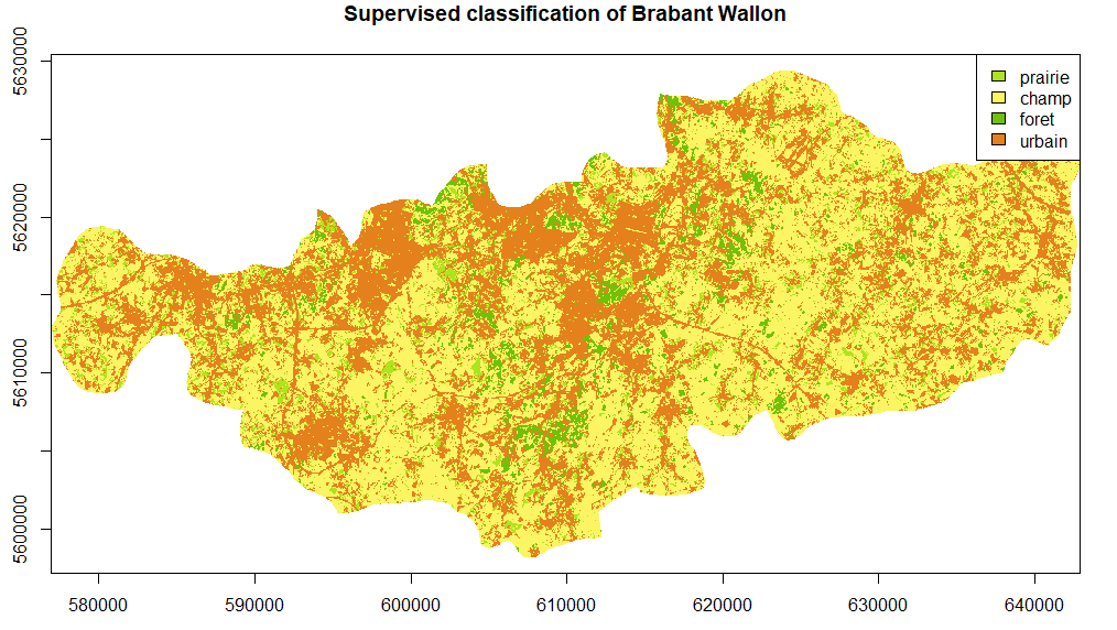
Unsurprisingly, the results are already much better. Fields occupy most of the territory. Grasslands and forests are rarer. Large urban areas can be easily distinguished and major roads such as highways are even noticeable. The confusion matrix and the kappa index also show good results. However, caution should be exercised due to the low number of observations.

Second case study: Greater London (leveraging the geo-wiki database)

In the second example, we will perform land cover classifications in the Greater London area. First, all bands from a set of Landsat 5 images are imported and stacked. A spatial object of the region is also downloaded.

#import and stack satellite images
landsatLD<-stack()
for (i in 1:2){
	name <- paste0('landsatLD',i)
	assign(name, raster(paste0('imagesLondon/LT05_L1TP_201024_20110930_20200820_02_T1_B',i,'.tif')))
	landsatLD<-stack(landsatLD,eval(parse(text=name)))
}
#import spatial object of the region of study
uk <- raster::getData("GADM", country = 'GBR', level =2, download=TRUE)
uk_sf<-st_as_sf(uk)
london_sf<-uk_sf[uk_sf$NAME_2=="Greater London",7]

Then we call the function specifying the unsupervised classification without providing the optional input. The function will use the geo wiki database to perform the validation.

#call function without optional arguments for unsupervised classification
output<-classification(images=landsatLD, smoothing = TRUE, window = 3,region = london_sf,type = 'unsupervised',k=4)
output
#plot
plot(output[[1]], main='Unsupervised classification of Greater London',legend = FALSE, col = c('#E4811D','#E4811D','#E4811D',"#70C108"),xlab = "Longitude (m)",  ylab = "Latitude (m)")
legend("topright", legend = c('urban','urban','urban','treecover'), fill = c('#E4811D','#E4811D','#E4811D',"#70C108"))

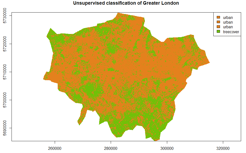
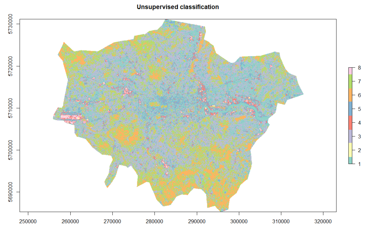
Note that there are only two classes whereas the call to the function required four classes. In fact, given the nature of the unsupervised classification and the “ultra-urban” character of central London, the algorithm distinguished between different types of urban areas before distinguishing urban areas from other classes (this is related to the advice to request more classes than necessary and gather them after the classification). Therefore, three different types of urban areas were manually grouped into one class. Asking for 8 classes as in the next map would give better end results but would require more post work to interpret the different classes.

Finally, a supervised classification of the same region, using the geo wiki database as training and validation files, will be carried out.

#call function without optional arguments for supervised classification
output<-classification(images=landsatLD, smoothing = TRUE, window = 3,region = london_sf,type = 'supervised')							
output

## $classification
## class      : RasterLayer 
## dimensions : 1528, 1983, 3030024  (nrow, ncol, ncell)
## resolution : 30, 30  (x, y)
## extent     : 255765, 315255, 5685315, 5731155  (xmin, xmax, ymin, ymax)
## crs        : +proj=utm +zone=31 +datum=WGS84 +units=m +no_defs 
## source     : memory
## names      : lyr.1 
## values     : 1, 4  (min, max)
## 
## 
## $kappa_index
## [1] 0.9083333
## 
## $confusion_matrix
##                 cultivated       urban grassland treecover water
## cultivated           7.000   6.0000000         3         0     0
## urban                0.000 113.0000000         0         0     0
## grassland            1.000   0.0000000         0         0     0
## treecover            0.000   1.0000000         0         0     0
## water                0.000   0.0000000         0         0     0
## inclusion_error      0.875   0.9416667         0       NaN   NaN
##                 exclusion_error
## cultivated            0.4375000
## urban                 1.0000000
## grassland             0.0000000
## treecover             0.0000000
## water                       NaN
## inclusion_error       0.9160305
## 
## $class_order
## [1] "cultivated" "urban"      "grassland"  "treecover"  "water"

#plot
plot(output[[1]], main='Supervised classification of Greater London',legend = FALSE, col = c('#FBF463','#E4811D','#AEE41D',"#70C108"),xlab = "Longitude (m)",  ylab = "Latitude (m)")
legend("topright", legend = output[[4]], fill = c('#FBF463','#E4811D','#AEE41D',"#70C108",'blue'))

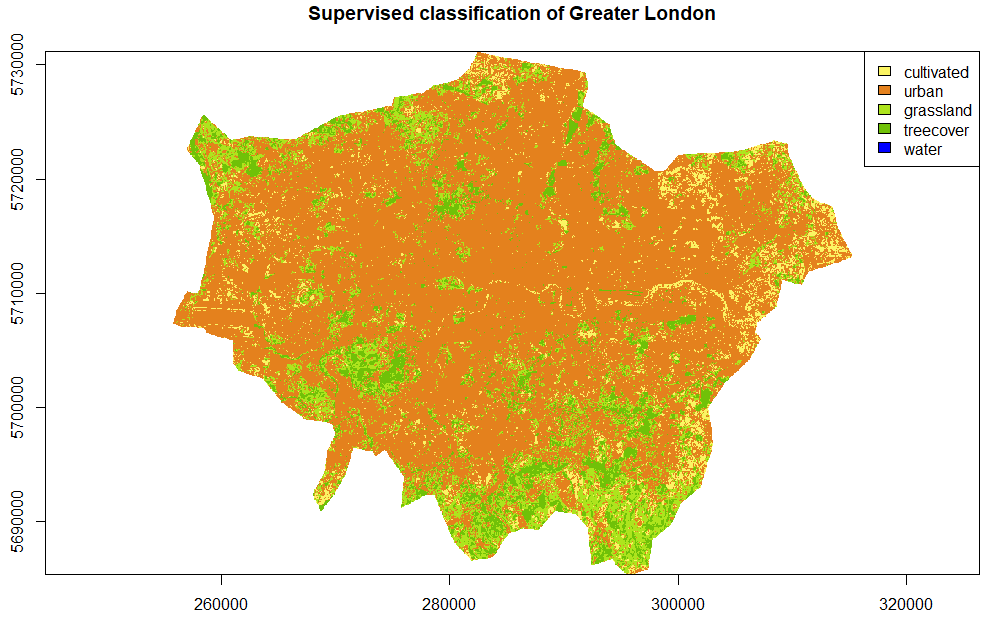
The result obviously strongly depends on the database used to train the model. However, among the four hundred observations made in the region, only one concerned the “water” class. This explains why this class is so poorly represented, e.g. the River Thames is clearly visible and has been assigned to cultivated areas. Better results could not be expected with so few observations! As a reminder, the objective here was to demonstrate that a certain level of automation has been achieved and that the results could be easily improved only by having access to one or more additional databases and by choosing more carefully satellite images.